
Forecasting Sales using Statistical Models
In « How do I use Statistical Models to Forecast Sales? », published by Forecast Pro, you will find an excellent description of the main statistical methods and techniques to forecast any variables. All these methods are integrated in the latest version of Forecast Pro Trac 6.
Sales and demand forecasters have a selection of techniques at their disposal to predict the long run. While most analysts will examine historical sales or other sorts of knowledge as a guide, many forecasters rely heavily on judgment. There’s little question that judgment can play an enormous role in arriving at your final, consensus forecast – but statistical forecasting offers A level of automation and insight which can substantially improve your forecast accuracy, particularly once you’re producing large quantities of forecasts on a rolling basis.
In this article, Forecast Pro covers two common approaches for forecasting sales using statistical methods: statistic models and regression models. The advantage of these approaches is that they supply plenty of “bang for your buck”. On one hand, they’re robust methods which can detect and extrapolate on patterns in your data like seasonality, sales cycles, trends, responses to promotions, and so on. On the other hand, they’re easily accessible approaches, especially with the right tools.
Time Series Methods
Time series methods are forecasting techniques that base the forecast solely on the demand history of the item you’re forecasting. They work by capturing patterns within the historical data and extrapolating those patterns into the long run. Statistic methods are appropriate once you’ll assume a cheap amount of continuity between the past and thus the longer term. They’re best suited to shorter-term forecasting (for example, projecting out 18 months or less). This is often often because of their assumption that future patterns and trends will resemble current patterns and trends. this is often often a cheap assumption within the short term but becomes more tenuous the further out you forecast.
Common Time Series Models
- Very simple models.Moving averages, “same as last year”, percentage growth and best-fit line (i.e., regression against time) are all very simple time series models that can be used to generate forecasts. They can be implemented in a spreadsheet in a matter of seconds and do not require any statistical expertise on the part of the forecaster; however, for most business applications these methods are too simple and more accurate forecasts can almost always be generated using alternative time series methods.
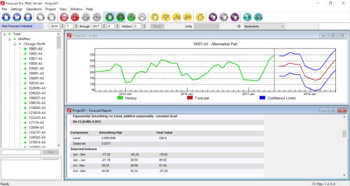
- Exponential smoothing models.Exponential smoothing is the method of choice for many corporate forecasters. The models perform well in terms of accuracy, are easy to apply and can be automated, allowing them to be used for large scale forecasting. Exponential smoothing models capture and forecast the level of the data along with different types of trends and seasonal patterns. The models are adaptive and the forecasts give greater emphasis to the recent history vs. the more distant past.
Box-Jenkins (ARIMA) models. Box-Jenkins models are almost like exponential smoothing models therein they’re adaptive, can model trends and seasonal patterns, and should be automated. They differ therein they’re supported autocorrelations (patterns in time) rather than a structural view of level, trend and seasonality. Box-Jenkins models tend to perform better than exponential smoothing models for extended, more stable data sets and not also for noisier, more volatile data.
- Croston’s intermittent demand model.The Croston’s model is specifically designed for data sets where the demand for any given period is often zero and the exact timing of the next order is not known. Low-level data (e.g., SKU by customer) or spare parts often exhibit this kind of demand pattern. This method works by combining a smoothed estimate of the average demand for periods that have demand with a smoothed estimate of the average demand interval. The forecasts are not magic (they won’t tell you when the next order will be placed); however, they often yield a better forecast for expected demand than other time series approaches.
Building Time Series Model
While many of these models can be built in spreadsheets, the fact that they are based on historical data makes them easily automated. Software packages can build large amounts of these models automatically across large data sets. In particular, data can vary widely, and the implementation of these models varies as well, so automated statistical software can assist in determining the best fit on a case by case basis.
Regression Models
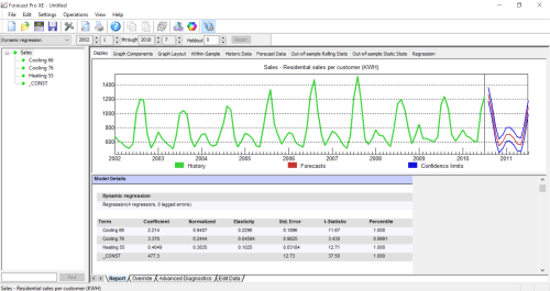
Dynamic regression models allow you to incorporate causal factors such as prices, promotions and economic indicators into your forecasts. The models combine standard OLS (“Ordinary Least Squares”) regression (as offered in Excel) with the ability to use dynamic terms to capture trend, seasonality and time-phased relationships between variables. The result is a model that will forecast more accurately than straight time series approaches when explanatory variables are driving the demand for your products or services and certain other conditions are met.
A well-specified dynamic regression model lends considerable insight into relationships between variables and allows for “what if” scenarios. For instance, let’s say that your dynamic regression model includes price as an explanatory variable. By quantifying the relationship between sales and price, the model allows you to create forecasts under varying price scenarios. “What if we raise the price?” “What if we lower it?” Generating these alternative forecasts can help you to determine an effective pricing strategy.
The “what if” analysis described above hints at the biggest drawback to using dynamic regression. A well-specified dynamic regression model captures the relationship between the dependent variable (the one you wish to forecast) and one or more independent variables. In order to generate a forecast, you must supply forecasts for your independent variables. If these independent variables are under your control (e.g., prices, promotions, etc.) or if they are leading indicators, this may not be a big issue. If, however, your independent variables are not under your control (e.g., weather, interest rates, price of materials, competitive offerings, etc.) then you need to keep in mind that poor forecasts for the independent variables will lead to poor forecasts for the dependent variable.
Building a Regression Model
While there are software tools out there that can automate time series forecasting very effectively, regression is usually a bit different. It is a method where knowledge of the technique and experience building the models is quite useful. Building a dynamic regression model is generally an iterative procedure, whereby you begin with an initial model and experiment with adding or removing independent variables and dynamic terms until you arrive upon an acceptable model. Tools like Forecast Pro provide a complete range of self-interpreting hypothesis tests and other diagnostics to help guide you through the process.
Conclusion
Statistical methods can provide a level of automation and accuracy that purely judgmental methods simply can’t provide on their own. Not only can these models help you identify recurring patterns and trends in your data, they can also save you tons of time and effort by automatically forecasting big data sets, and as a result you can direct your focus to where your judgment counts the most.